|
The Art of Demomaking - Issue 08 - Fractal Zooming by (11 October 1999) |
Return to The Archives |
Introduction
 |
|
Well this is the 8th tutorial! I'm glad to see you got so far. For those of you that can remember, the original plan was to split the tutorial into two series, but I've changed my mind. I'll just keep on writing until I run out of techniques to explain. Obviously I could go on for a while explaining every single effect in the book, but I'd get bored of that pretty quickly, and there wouldn't be anything left for you to do ;) And besides, with the knowledge you have now you should be able to code virtually any effect you think of. If not, then hack your way around the problem... that's what it's all about! This week we are going to learn about zooming, and what best to zoom than an infinite fractal?? Don't worry if you know nothing about complex numbers, all will be explained. I'll also show that there's nothing more to zooming than more interpolation. We will also cover dynamic mipmapping in this tutorial. |
|
Complex Numbers
|
Complex numbers can be split into two different components, the real part and the imaginary part. If the imaginary part is null, then the number is just like a normal real number. This is how a complex number is written:
a is the real part, and b is the imaginary part. i is the square root of minus one! If you've never heard of complex numbers before this may come as a shock... Indeed the square root of a negative number cannot be determined. And neither can i, which therefore has an undetermined value. The only thing you know is:
I suppose that's where the imagination comes into play :) However, there is an easier way to think of a complex number. You can place it on a graph, more commonly called the complex plane. The real part of a complex number is used as the X coordinate, and the imaginary part as the Y coordinate. Operations on complex numbers are quite straight forward. Just develop the equations as usual, and replace any occurrences of i*i with -1. Then refactorise to obtain the standard way to express complex numbers.
You could learn a lot more about complex numbers if you're interested in 2D algebra, but that's all we need to know to code our fractal. |
|
The Mandelbrot Fractal Set
|
The magic of fractals is that they can be generated to any zoom level with one single equation! In our case, for the mandelbrot set, the equation is:
A complex number C is said to belong to the mandelbrot set if Z(n) remains within finite distance of the origin when n is infinitely big. So basically, there are two types of complex numbers, those that belong to the mandelbrot set, and those that don't. What we have to do is to efficiently determine whether a complex number is in the mandelbrot set or not. Here's the trick. As soon as Z(n) goes beyond the circle around the origin of radius 2, then it has been proven that when n gets infinitely big, so will Z(n). So all we need to do is repeat the calculation of equation (1) until the distance between Z(n) and the origin is more than 2. Of course that may never happen, so we must add a simple counter to our loop, and bail out if the counter reaches a certain limit. Here's what an iteration looks like: 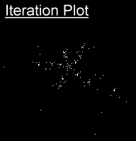 The problem is, there are only 2 kinds of complex numbers, either in or out the fractal set. So that's two colours to assign, which admittedly is quite boring. A simple hack is to use the value of the counter to reference a colour in the palette. Basically we assign a colour based on the number of iterations we needed to determine if C was in the set. This doesn't make much sense mathematically, but it looks really good ;) Rendering images of the complex plane is interesting for complex numbers in the range (-1.5,-1) to (0.5,1). You will recognise the beetle like shape, also known as cardioid, characteristic of the Mandelbrot fractal set. The further you zoom in, the more cardioids you find... I find it fascinating that a simple equation like that can produce such complex patterns! |
|
The Theory For Fractal Zooming
|
|
You could just calculate a zoomed fractal every frame, but that would take you a couple of seconds to render on fast computer. Calculating at a lower resolution would be quicker, but wouldn't look very nice. You could also gradually update each pixel in a pseudo-random order. This can look quite cool if you find a good order to render the pixels in. One of the simplest yet effective way I've come across is to render a fractal at twice the screen resolution, and zoom that while calculating the next fractal. You can get amazing FPS and high quality fractals. So the fractal algorithm just need to calculate bitmaps zoomed twice closer every time. 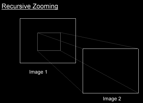 |
|
Zooming Bitmaps
|
There's absolutely nothing new here. It's just a question of interpolating our X and Y positions in the bitmap, and fetching the texels with optional bilinear filtering.
Some of you may have noticed that some texels irregularly appear and disappear while zooming. This is noticeable when the texels in question are a colour much different to neighbouring ones. This is due to the fact that we skip some texels in the bitmap while interpolating. Mipmapping was intended to prevent exactly this problem, but calculating a mipmap of our fractal would kind of defeat the point, since the fractal would end up being displayed at a lower resolution until the last frame of the zoom, when the algorithm would use the normal bitmap. This switch in mipmaps would look very obvious. The solution I came up with was dynamic mipmapping, which I implemented into the code. It worked, but the code was quite bulky, the zooming loop ran about 50% slower and it didn't make that much difference at all, so I dropped the idea. I'll still explain the concept, for those of you that are interested. All we need to do is to find what area of each texel is covered by the pixel, and calculate a weighted average of the texels underneath: 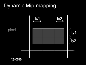 The tricky part is that a pixel can cover 2x2, 2x3, 3x2, and 3x3 texels. So either you load all 9 texels every time, or you implement a simple if statement, to handle each case separately. This prevents loading texels unnecessarily, but the code looks very unpleasant ;) I'll just give you the code for the 2x3 case, the others are pretty straight forward from then on.
pixelsize remains constant for each pixel. You just need to compute it once per call to the zooming procedure. It's a 16.16 fixed point variable. You can implement dynamic mipmapping if you feel up to it, but keep in mind it will slow your loop down quite a bit. Things will look better, and less texels will randomly appear. But I personally believe that the quality of bilinear filtering is not that far away in most cases, except in high contrast areas. |
|
Final words
|
|
Fractals are often used in computer art, and can produce some fascinating images. They are also quite common in realtime demos, where they can produce some impressive effects. And it just keeps on going.... our poor computers can only compute an infinitely small portion of the fractal! Zooming can be used without fractals, for simple pre-rendered bitmaps for example. As you noticed, there's nothing difficult to it, it's just more interpolation. Dynamic mipmapping on the other hand can get a bit harder, but the results do reflect the work put in to implement it. Next week we will talk about textured screens, like in tunnels and flowers. We will also learn about profiling, and a bit of assembler. It makes a nice change to know for sure what's going to happen next week ;) But don't get used to that... I like being unpredictable! Download this week's demo and source code package right here (67k) Happy coding, Alex |